Proof of Concept: Python

![]()
![]()
![]()

All Project Files are located in my GitHub Repository
Plotting Static Figures
Import Relevant Packages
import pandas as pd
import matplotlib.pyplot as plt
import numpy as np
import os
Declaration of Variables
Enter the relative path to data:
data_path = 'data/'
fig_location = 'plots/'
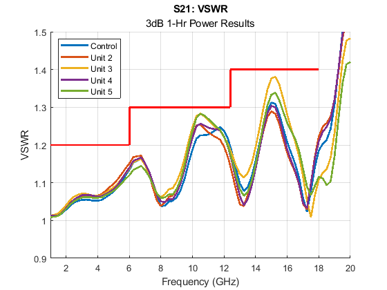
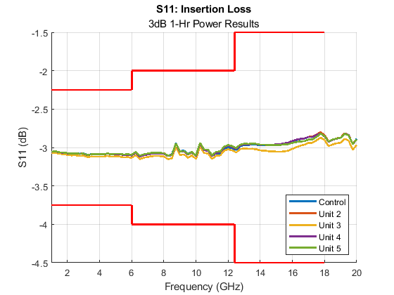
s_parameter = ['VSWR', 'S21(db)']
delimiter = ','
output_plot_figures = ['VSWR ','Insertion Loss ']
y_smooth = np.array([])
Function Definitions
Retrieve File Paths:
def get_file_paths(data_folder):
    list_csv_files = []
    file_index = []
    paths = []
    for root, folders, files in os.walk(data_folder):
        files = [f for f in files if not f[0] == '.']
        folders[:] = [d for d in folders if not d[0] == '.']
        if files == []:
            continue
            for index, value in enumerate(files):
            list_csv_files.append(value)
            file_index.append(index)
            p = root + value
            paths.append(p)
    return file_index, list_csv_files, paths
Read All CSV Files in A Directory:
def funct(paths,i):
    figure, ax = plt.subplots(figsize=(11,8))
    for index, value in enumerate(paths):
    df = read_files(value)
    plot_data(df,index)
    ax = format_axes(ax,i)
Read CSV Files into Pandas Data Frame:
def read_files(list_csv_files):
    cols = ['Point', 'Frequency', 'VSWR','f2', 'S21(db)']
    df = pd.read_csv(list_csv_files,
        skiprows=17,
        delimiter=',',
        header = None,
        names = cols,
        )
    if any(df['VSWR'] < 1) :
        df['VSWR'] = (10**(-df['VSWR']/20) + 1) / (10**(-df['VSWR']/20) - 1)
    return df
Plot Data:
def plot_data(df,dut_num):
    str1 = ['Pre-Power','Post-Power','Post-Thermal Shock', 'Orginal Springs', 'Post-Power 2019']
    x = df['Frequency']
    y = df[s_parameter[index]]
    label_name = str1[dut_num]
    plt.plot(new_x,
        y_smooth,
        'r-',
        label=label_name,
        )
Format Plots:
def format_axes(ax,figure_index):
	  xlabel = 'Frequency'
    ylabel = s_parameter[figure_index]
    fig_title = output_plot_figures[figure_index]
    plt.rc('lines', linewidth=2)
    ax.set_title(fig_title)
    ax.set_xlabel(xlabel)
    ax.set_ylabel(ylabel)
    ax.grid(color='grey', linestyle='-', linewidth=0.25, alpha=0.5)
    ax.spines['top'].set_visible(False)
    ax.spines['right'].set_visible(False)
    ax.legend()
Main Program
file_index,files,paths = get_file_paths(data_path)
for index, value in enumerate(output_plot_figures):
    funct(paths,index)
    fig_location = 'graphs/' + value
    plt.savefig(fig_location)
Static Examples with Random Created Data
Plotting Dynamic Figures
Interactive Plots using the Bokeh Library.
Import Relevant Packages
import pandas as pd
import numpy as np
import os
import matplotlib.pyplot as plt

from bokeh.io import output_file, output_notebook, export_png
from bokeh.plotting import figure, show
from bokeh.models import ColumnDataSource, NumeralTickFormatter, HoverTool,  PrintfTickFormatter
Declaration of Variables
cols = ['Frequency', 'VSWR', 'S11(DB)','a ',' b',' c',' d',' e','h']
data_path = 'data/'
Function Definitions
Retrieve File Paths:
def get_file_paths(data_folder):
    list_csv_files = []
    file_index = []
    paths = []
    for root, folders, files in os.walk(data_folder):
        files = [f for f in files if not f[0] == '.']
        folders[:] = [d for d in folders if not d[0] == '.']
        if files == []:
            continue
        for index, value in enumerate(files):
            list_csv_files.append(value)
            file_index.append(index)
            p = root + value
            paths.append(p)
    return file_index, list_csv_files, paths
Read All CSV Files in A Directory:
def plot_figures(df,ax):
    df.plot(ax=ax,
            x='Frequency',
            y='VSWR',
           )
Main Program
Call Funaction Definitions & Set Interactive Tools:
file_index,files,paths = get_file_paths(data_path)
fig, ax1 = plt.subplots(figsize=(11,8))
select_tools = ['box_select', 'lasso_select', 'poly_select', 'tap', 'reset', 'wheel_zoom', 'box_zoom']
linecolor = 'royalblue','green','red'
DUT = 'DUT1', 'DUT2','DUT3'
Format Plot Figure:
fig = figure(plot_height=820,
             plot_width=1800,
             x_axis_label='Frequency (GHz)',
             y_axis_label='VSWR',
             title='VSWR',
             toolbar_location='below',
             tools=select_tools,
            )
Read CSV Files:
for index, value in enumerate(paths):
    df = pd.read_csv(value,
        # skiprows=8,
        delimiter=',',
        # header = 19,
        names = cols,
        )
    if any(df['VSWR'] < 1) :
        df['VSWR'] = (10**(-df['VSWR']/20) + 1) / (10**(-df['VSWR']/20) - 1)
    x= df['Frequency']
    y = df['VSWR']
    plot_figures(df,ax1)
Configure Data Frame as a Bokeh Object:
    data_cds = ColumnDataSource(df)
    fig.line(x='Frequency',
            y='VSWR',
            source=data_cds,
            color=linecolor[index],
            selection_color='deepskyblue',
            nonselection_color='lightgray',
            nonselection_alpha=0.3,
            legend_label=DUT[index],
            line_width=2.0,
            )
Format and Output HTML File:
output_file('DynamicGraph.html', title='Jose\'s Dynamic Graphing Skills!!')
output_notebook()

fig.title.align = 'center'
fig.xaxis[0].formatter = PrintfTickFormatter(format="%1.0f")
fig.yaxis[0].formatter = NumeralTickFormatter(format='0.00')
fig.legend.title = 'DUT\'s'
fig.legend.location = 'top_left'
fig.add_tools(HoverTool(
    tooltips=[
              ( 'Frequency',   '$x GHz'),
              ( 'VSWR',        '@{VSWR}' ),
             ],
    formatters={
                '@{Frequency}' : 'numeral',
                '@{VSWR}' : 'numeral',
                },
    mode='vline'
                        )
                )
show(fig)